Gausiann Process Are a (giant) Box of Functions

If you work in autonomous experimentation, chances are you have encountered the term Gaussian Process more times than you would care to admit. Even if you are not entirely sure what the process is, or what exactly is Gaussian about it, you probably know that it is a model that gives you a prediction and some measure of uncertainty for the input–output relationship you are trying to learn.

What is funny to me is that almost every paper that uses a Gaussian Process—including papers claiming to use it on some kind of materials data “for the first time ever” (honestly, why should anyone care?)—seems to include an unnecessary amount of mathematics copied directly from textbooks.

I have written mathematically heavy papers and published them in materials science journals, so I know how difficult it can be to convince reviewers that all of that mathematical machinery is actually necessary. I completely understand including the mathematics when you are making a genuine scientific contribution that requires the reader to understand the underlying formulation. Even if the only person who benefits from those equations is a single PhD student somewhere in Buffalo, NY who finally understands the mathematical underpinnings of the method, that can be worthwhile.

But often, I see these sections presented as pure copy-and-paste exercises: a way to fill up space and make the paper look more “complete.” If you are using a method that has already been formalized in textbooks and implemented in well-established software packages, I am not sure reproducing the entire mathematical formulation necessarily helps the reader understand what you actually did with it.

And that brings me to another aspect of Gaussian Processes that I have seen creep into the materials data-science community: the kernel function.

Uff.

Why are we so obsessed with kernels as if they are simultaneously the savior—and the fundamental problem—of applying GPs to materials data?

I get it. It is fashionable to say that something is “physics-informed,” and one way of doing that is to use a kernel that is different from the good old RBF or Matérn kernel because it supposedly captures something special about the input–output relationship.

But isn’t that exactly the point of using a GP?

Anyway, I will stop ranting about GPs for a moment and try to explain a viewpoint that helped me completely bypass what I like to call the GP kernel cartel.

The same idea applies to the “physics-informed” mean function.

I like to think about a Gaussian Process as a box of functions.

A particular combination of a mean function and a kernel defines a probability distribution over functions. In other words, you have a box containing a very specific family of possible functions that could represent the input–output relationship you are trying to model.

Now imagine a shelf containing many such boxes. Each box corresponds to a different GP: different mean functions, different kernels, different assumptions about how the output should vary as a function of the input.

You can choose one of these boxes. Or, if you are sufficiently ambitious, you can build your own by combining different ingredients to create a broader or more appropriate family of functions.

But for now, let’s forget all the mathematical wizardry and just think about the box of functions.

When you fit a GP to a set of input–output observations, you are effectively asking:

Which functions inside this box are consistent with the data I have observed?

Before seeing any data, many of the functions in your box may be plausible. Once you observe a few data points, some functions become much more plausible than others, while others become essentially impossible. This is your posterior distribution over functions.

With only a handful of observations, there may still be a huge number of functions that explain what you have seen. As you collect more observations, the set of plausible functions gets progressively narrower.

And this is where the familiar GP prediction and uncertainty come from.

The mean of the posterior distribution over functions gives you the GP prediction. The covariance of that posterior distribution tells you how much those plausible functions disagree with one another—and therefore gives you a measure of uncertainty about the latent function you are planning to model.

This viewpoint is particularly useful because it immediately leads to an important clarification about what GP uncertainty actually means.

What uncertainty are we talking about?

One of the most unfair criticisms—or perhaps misunderstandings—of GPs in materials science concerns uncertainty quantification.

By definition, the uncertainty produced by a GP is primarily uncertainty about the function you are trying to infer from your input–output observations.

It is not automatically the uncertainty associated with the data collection process itself.

Those are different things.

Suppose I measure the phase behavior of a material and obtain an observation ($y$) at some experimental condition ($x$). There may be uncertainty because I do not know the underlying function that maps $x$ to $y$. But there may also be uncertainty because my instrument is noisy, my sample preparation is imperfect, or the experiment itself has stochastic variability.

The GP’s likelihood provides a way to model this observation noise. The kernel, in contrast, primarily describes assumptions about the correlations and smoothness of the underlying function.

This distinction matters when people say they want “quantified uncertainty.” Are they asking:

How uncertain am I about the underlying function?

or:

How noisy is the measurement process?

These are not necessarily the same question.

There is also an important practical complication. Many of the convenient analytical methods for fitting GPs rely on a Gaussian likelihood. Once you move to non-Gaussian observation models, inference becomes substantially more complicated.

So the next time you fit a GP and find yourself endlessly playing around with kernels, do yourself a favor:

Plot samples from the distribution over functions defined by your mean and kernel.

Take a peek inside the box.

For one-dimensional functions, this is relatively easy to visualize—and 1D functions are almost never the things we actually care about in materials science.

I often wish there were a cleaner way to visualize this in two or three dimensions. Imagine being able to look at a set of sampled phase maps from your GP and literally see the kinds of phase diagrams that your model believes are plausible.

That would make my work considerably more visual.

The kernel is the problem formulation, not the solution

The only time I feel I really used this “box of functions” viewpoint effectively was in a paper where we developed a probabilistic classifier for two sets of curves: one exhibiting stationary behavior, where the shape is locally correlated and the kernel can be expressed as a function of distance, and another exhibiting non-stationary behavior, where correlations are more complicated and cannot be captured by distance alone.

I was pretty happy with that work because, in some sense, it was exactly what the GPML book told me to do.

At the time, I was still learning what GPs really were. My favorite ML teacher of all time said in his YouTube video lectures once to not to worry too much about thinking about GPs as distributions over infinite-dimensional function spaces.

I agreed with him.

In fact, infinite dimensional function spaces aka Hilbert spaces are a very fundamental concept that shaped how my postdoctoral research evolved but it never really helped me understand GPs any better. It is mathematically elegenat but then has the same problem as the kernel cartel math.

Years later, I was at an MRS conference listening to a talk about how non-stationary kernels were going to fundamentally change the way we solve materials optimization problems.

And I remember thinking:

Finding the right kernel is the problem formulation, not the solution.

That, to me, is the key point.

A kernel encodes assumptions about the kinds of functions you are willing to consider plausible. Choosing one is therefore an important modeling decision. But it is not, by itself, a scientific solution to a materials optimization problem. So don’t advertise it as one.

We should absolutely build better kernels when the scientific problem demands them. We should incorporate physical knowledge when we have it. We should develop models that capture structure that generic kernels cannot.

But perhaps we should stop treating the kernel as the hero of the story.

The interesting question is not:

Which kernel should I use?

It is:

What family of functions do I believe could plausibly describe my materials system—and how can I efficiently learn which functions within that family are consistent with my experiments?

Once you start thinking about GPs that way, the kernel becomes much less mysterious.

It is simply a way of defining the box. So you can finally ask the question: what’s in the box?

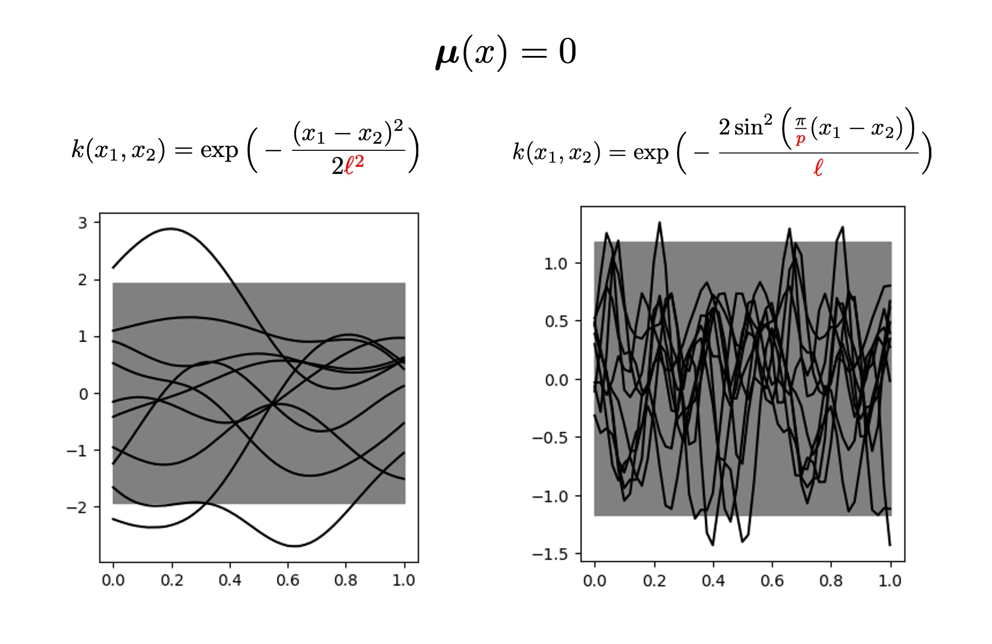
Figure 1. A Gaussian Process can be viewed as a probability distribution over a “box” of plausible functions.